How I Built an Image Classifier with Absolutely No Machine Learning

“This solution looks promising but let us get back to you. The investment of deploying this solution might be a bit too high.”

I was disappointed. We all knew what that eventually means.

How could we not think of it? We were over-focused on the accuracy and performance of the solution, we ignored the infrastructure costs.

That is when I realized I need to learn and apply traditional image processing techniques that don’t demand a lot of computing and infrastructure cost as much as advanced machine learning approaches but still delivers performance to an acceptable level.

So how do we solve problems using traditional image processing? I’m no computer vision expert, but I learned a few things I’m about to share with you.

Portfolio Project: Day-Night Image Classifier

For obvious reasons, this isn’t the same problem I talked about earlier, but let’s say it’s somewhat similar.

We build a simple classifier that, given an image, can correctly identify if it’s a day or a night image. Most real-world vision-based systems are required to distinguish between day and night.

Having adopted this as one of my portfolio projects, I’ve received continuously positive interviewers' responses around the underlying thought process. I am confident you would benefit from adopting this to your portfolio.

This project's data is an extract of 400 images from the AMOS dataset (Archive of Many Outdoor Scenes). These are RGB colored and contains 200 each of day and night classes—credits to Udacity for putting together this project in their Computer Vision Nanodegree, which I graduated.

The codes that follow, including the dataset, can be found in the GitHub repository. Forking the repository would give you everything you’ll need to follow along.

I’ve taken a 5 step approach with clear explanations for each one of them. By the end of the article, you’ll have an in-depth understanding of the computer vision pipeline employed for this project.

Let’s get started?

Step 1: Load and visualize the data.

We have a set of images in the directory. Our task is to load it conventionally and their labels, such that it can be used to visualize and later build the classifier.

In Python, the glob module is used to retrieve files/pathnames matching a specified pattern. Using matplotlib’s image module, we can read load images into memory.

We need to visualize to understand the data better. Passing the relevant directory to the function above will load the data, and using matplotlib’s imshow() function, we can visualize the images. Having a sound understanding of the data is only going to help you down the pipeline.# Load training data
IMAGE_LIST = load_dataset(image_dir_training)# Select an image and its label by list index
image_index = 49
selected_image = IMAGE_LIST[image_index][0]plt.imshow(selected_image);

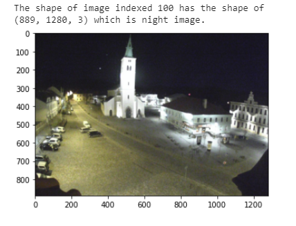
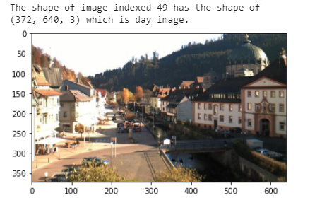
• Notice any measurable differences between these images? This can help later separate the image classes.
• Notice how different images are of different sizes? This isn’t ideal when you want to apply any image processing (or deep learning).

Step 2: Preprocess the data.

Pre-processing is crucial when it comes to all sorts of vision problems. Due to varying levels of light and other factors when an image is captured, often images aren’t uniform, making it hard to extract features.

Let’s work on basic pre-processing such as standardizing the image sizes and encoding the images' labels.

The code is self-explanatory. We resize all images to a standard size of (1100,600). It’s not mandatory to choose this shape, but whichever shape you choose needs to be constant throughout the project.

Most classification problems require us to have the target classes in numerical format. We can use encoding to achieve this—a simple one-hot encoding where 1 for day and 0 for night images could be used.

We wrap the encode()and standardize_input() functions into the preprocess() function and use it to standardize our images. Now that we have loaded and pre-processed our images, we are literally in good shape to extract features out of the images (the interesting part of the pipeline!).

Step 3: Extract the features.

To extract features from the images, we need to understand some basic properties of images.

We need to extract such features that can distinguish the day images from night images. When you approach a classification challenge, you may ask yourself: how can I tell these images apart?

The feature that occurred to my mind is most day images had bright blue skies and is generally more radiant. In night images, the only light source was some artificial lights, and the background is comparatively darker.

We can take this property and see if we can measure it to become a feature that could separate the classes.

Average Brightness as a Feature

To quantify the average brightness of an image, we need first to understand color spaces. When I first heard of this concept, I was confused, so please slow down and read this with more attention.

Treating images as grids of numbers is the basis for many image processing techniques. Every pixel in an image is just a numerical value and, we can also change these pixel values. These pixels have one single color, which is represented by a color space.

The most common color space is RGB, which stands for 3 channels red, green, and blue. So every pixel in an image can be represented using these 3 numbers in RGB color space. But there are other color spaces too which can be useful.

For instance, another color space is HSV — standings for Hue, Saturation, and Value. These 3 component vary with various things of an image:

• Hue stays consistent under shadow or even under high brightness.
• Value varies the most under different lighting conditions.
• Saturation describes the amount of gray in a particular color.

With that information, we can now go back to deriving the average brightness. How? Here are the steps we would follow.

1. Convert the image to HSV color space (as we explained above, Value channel is an approximation for brightness)
2. Sum up all the values of the pixels in the Value channel
3. Divide that brightness sum by the image area, which is just the width times the height.

This gave us one value: the average brightness of the image. This is a measurable value and can be used as a feature for the classification problem at hand. Let’s implement the steps in a function.

We can create more features, but for this example, let’s keep it simple. Now that we have a feature, I can’t wait to build the classifier along with you.

Step 4: Build the classifier.

We have been so used to advanced machine learning algorithms; we forget the primary function of a classifier. It is to separate two classes. We defined one feature, and we need a way to separate the image based on the feature.

A classifier can be as simple as a conditional statement that checks if the average brightness is above some threshold, then this image is labeled as 1 (day), and if not, it’s labeled as 0 (night).

Let’s implement this function, shall we?

There’s a catch, though, what is an acceptable threshold value? Normally we seek domain experts' advice to understand these values, but here since we have sufficient training images, we can use them to estimate one.

Our next task is to tweak the threshold, ideally somewhere in the middle of 0–255. I tried different values and checked with various training images to see if I have classified the images correctly. In the end, I settled for 99.

Now that we have built a classifier let’s see how we can evaluate the model?

Step 5: Evaluate the classifier.

Every model needs to be evaluated on unseen data. Remember the data we kept aside for testing? We need to run the test images through the classification and evaluate the accuracy of the model.

To find the accuracy of the model, we need to find the count of misclassified images. Doing this fairly straightforward. We write a function that takes the images with the real labels and the threshold, predicts the labels using the classifier, and compares it with the actual label.

Now that we have written the function, we need to ensure the test images are pre-processed the same way as we did for the training images.

Did you know the final accuracy value I got? A staggering 93.75%! Depending on the threshold value you chose previously, this value may fluctuate, so feel free to tweak the parameter and experiment with it.

An improvement to this would be to create more features from the image and add them to the classifier to make the more robust classification.

Now I know this was a simple problem with a much smaller dataset; however, it shows that we still can solve computer vision problems without using expensive advanced machine learning algorithms. Sometimes traditional image processing is all you need.

Final Thoughts

We looked in a computer vision pipeline for a portfolio project of the day-night classifier. We used a step by step approach throughout the pipeline to build this classifier.

• Loading and visualizing the data
• Pre-processing the data
• Extracting features
• Building a classifier
• Evaluating the classifier

We implemented the code throughout the article, and the compiled version is available in the GitHub repository.

Thank you for following along in the article to the very end; if you’ve got any questions or feedback, feel free to say a Hi on LinkedIn.

The project's whole point is to demonstrate value in traditional approaches and realize advanced machine learning isn't always the way to go.

This is a reality check on ourselves where we tend to go for advanced machine learning approaches since it often results in higher performance, but often at the expense of expensive compute power.

Now I explore various approaches and evaluate trade-offs between explainability, infrastructure, performance, and cost before developing a product.

I like to think I'm becoming a better data scientist.

For more helpful insights on breaking into data science, interesting collaborations, and mentorships, consider joining my private list of email friends.